ESM_project

Path model

The tested path model Figure 1. Hypothesised path model

Code

# Import the data
#| include: false
#| message: false
#| warning: false
#| echo: false
cd<-getwd()

# file dir
file_dir<-"Originaldatensätze/R-Skript"

# young adults' dataset
YA_df<- read_spss(paste0(file_dir, "/ExpSamp_jungErw2.sav"))

# rename the age group
YA_df$agegroup<-"YA"

# check task_monitoring
hist(YA_df$esm_day_task_monitoring)

Code

# middle-aged adults
MAA_df<-read_spss(paste0(file_dir, "/ExpSamp_mittlErw.sav"))

# rename the age group
MAA_df$agegroup<-"MAA"

# check task_monitoring
hist(YA_df$esm_day_task_monitoring)

# combine the two
all_df<-rbind(YA_df, MAA_df)

Participants

Code

all_df %>%
  distinct(ID, agegroup) %>%
  count(agegroup, name = "n_participants") %>%
  gt() %>%
  tab_header(
    title = "Participants by age group"
  )

agegroup	n_participants
Participants by age group
MAA	103
YA	107

Code

# check the length of unique IDs
length(unique(all_df$ID))

[1] 210

the df looks like this:

# A tibble: 20 × 15
   ID         day  time intention                esm_day_stress esm_day_business
   <chr>    <dbl> <dbl> <chr>                             <dbl>            <dbl>
 1 AM05UN20     1     1 Brief abgeben                         3                2
 2 AM05UN20     1     2 Brief abgeben                         4                3
 3 AM05UN20     1     3 Brief abgeben                         4                5
 4 AM05UN20     1     4 Brief abgeben                         4                4
 5 AM05UN20     1     5 Brief abgeben                        NA               NA
 6 AM05UN20     1     1 Präsentation fertigstel…              3                2
 7 AM05UN20     1     2 Präsentation fertigstel…              4                3
 8 AM05UN20     1     3 Präsentation fertigstel…              4                5
 9 AM05UN20     1     4 Präsentation fertigstel…              4                4
10 AM05UN20     1     5 Präsentation fertigstel…             NA               NA
11 AM05UN20     1     1 Geschwister treffen                   3                2
12 AM05UN20     1     2 Geschwister treffen                   4                3
13 AM05UN20     1     3 Geschwister treffen                   4                5
14 AM05UN20     1     4 Geschwister treffen                   4                4
15 AM05UN20     1     5 Geschwister treffen                  NA               NA
16 AM05UN20     2     1 Kaffe trinken gehen                   2                2
17 AM05UN20     2     2 Kaffe trinken gehen                   2                3
18 AM05UN20     2     3 Kaffe trinken gehen                   4                4
19 AM05UN20     2     4 Kaffe trinken gehen                   5                5
20 AM05UN20     2     5 Kaffe trinken gehen                   5                5
# ℹ 9 more variables: esm_day_task_monitoring <dbl>, esm_day_stress_avg <dbl>,
#   esm_daybusiness_avg <dbl>, esm_day_task_monitoring_avg <dbl>,
#   esm_evening_intention_importance_t1 <dbl>, esm_evening_off_loading <dbl>,
#   esm_evening_intention_execution <dbl>, age_group <dbl>, agegroup <chr>

Preprocessing

Rescale PM to range between 0 and 1

Code

all_df$esm_evening_intention_execution<-ifelse(all_df$esm_evening_intention_execution ==-1, 0, all_df$esm_evening_intention_execution)

Monitoring

Code

hist(all_df$esm_day_task_monitoring)

Code

# all_df$esm_day_task_monitoring_r<-ifelse(all_df$esm_day_task_monitoring ==-1, 0, 
#                                          ifelse(all_df$esm_day_task_monitoring== 0, 0, 1))

Rescale offloading

Code

hist(all_df$esm_evening_off_loading)

Code

all_df$esm_evening_off_loading_r<-ifelse(all_df$esm_evening_off_loading ==-1, 0,1)

hist(all_df$esm_evening_off_loading_r)

Reshaping

The dataset as it is now is good to test hypotheses on the variables that vary within day, e.g. stress, business, monitoring.
Reshape the dataset so there is only one unique intention per day, which is our base level.

RTeshaped dataset

`summarise()` has regrouped the output.
ℹ Summaries were computed grouped by ID and day.
ℹ Output is grouped by ID.
ℹ Use `summarise(.groups = "drop_last")` to silence this message.
ℹ Use `summarise(.by = c(ID, day))` for per-operation grouping
  (`?dplyr::dplyr_by`) instead.

# A tibble: 20 × 43
# Groups:   ID, day, intention [20]
   ID         day  time intention                esm_day_stress esm_day_business
   <chr>    <dbl> <dbl> <chr>                             <dbl>            <dbl>
 1 AM05UN20     1     2 Brief abgeben                         4                3
 2 AM05UN20     1     3 Geschwister treffen                   4                5
 3 AM05UN20     1     5 Präsentation fertigstel…             NA               NA
 4 AM05UN20     2     3 Freund besuchen                       4                4
 5 AM05UN20     2     5 Kaffe trinken gehen                   5                5
 6 AM05UN20     2     3 telefonieren                          4                4
 7 AM05UN20     3     1 Präsentation fertigstel…              2                3
 8 AM05UN20     3     3 aufräumen                             4                5
 9 AM05UN20     3     1 mit Freundin spielen                  2                3
10 AM05UN20     4     4 13 Uhr zum Geburtstag g…              4                5
11 AM05UN20     4     2 mit guter Laune aufsteh…              4                5
12 AM05UN20     4     5 nicht einschüchtern las…              3                2
13 AM05UN20     5     3 18 Uhr bereitmachen für…              4                5
14 AM05UN20     5     2 Motivation zeigen                     3                4
15 AM05UN20     5     3 ausschlafen                           4                5
16 AM05UN20     6     3 Praktikumsplatz suchen                4                4
17 AM05UN20     6     5 Präsentation fertigstel…              2                4
18 AM05UN20     6     1 mit Freunden treffen                  2                4
19 AM05UN20     7     1 Präsentation fertigstel…              5                5
20 AM05UN20     7     3 meinem Freund eine Freu…              4                4
# ℹ 37 more variables: esm_day_task_monitoring <dbl>, esm_day_stress_avg <dbl>,
#   esm_daybusiness_avg <dbl>, esm_day_task_monitoring_avg <dbl>,
#   esm_evening_intention_importance_t1 <dbl>, esm_evening_off_loading <dbl>,
#   esm_evening_intention_execution <dbl>, age_group <dbl>, agegroup <chr>,
#   esm_evening_off_loading_r <dbl>, mean_stress <dbl>, mean_business <dbl>,
#   grand_mean_esm_stress <dbl>, grand_sd_esm_stress <dbl>,
#   grand_mean_esm_day_business <dbl>, grand_sd_esm_day_business <dbl>, …

Distributions

Code

# Select the variables you want histograms for
df_selected <- stress_int_red %>%
  select(within_stress, within_importance, within_business, 
         within_off_loading, within_task_monitoring, 
         esm_evening_intention_execution,esm_day_task_monitoring,esm_evening_off_loading_r )

Adding missing grouping variables: `ID`, `day`, `intention`

Code

df_selected<-df_selected[, c("within_stress", "within_importance", "within_business", 
                             "within_off_loading", "within_task_monitoring", 
                             "esm_evening_intention_execution", "esm_day_task_monitoring", 
                             "esm_evening_off_loading_r")]

# Convert to long format
df_long <- df_selected %>%
  pivot_longer(cols = everything(), names_to = "Variable", values_to = "Value")

# Plot all histograms in one go using facets
ggplot(df_long, aes(x = Value)) +
  geom_histogram(bins = 30, fill = "grey70", color = "black") +
  facet_wrap(~ Variable, scales = "free") +
  theme_classic()

Warning: Removed 1952 rows containing non-finite outside the scale range
(`stat_bin()`).

Check the intraclass correlation coefficient (ICC)

Code

PM_YA <- glmer(esm_evening_intention_execution ~ 1 + (1 | ID), 
               data = stress_int[stress_int$agegroup=="YA",], family = binomial)

PM_MAA <- glmer(esm_evening_intention_execution ~ 1 + (1 | ID), 
                data = stress_int[stress_int$agegroup=="MAA",], family = binomial)

print("ICC PM YA:")

[1] "ICC PM YA:"

Code

icc_YA<-icc(PM_YA)
icc_YA$ICC_adjusted

[1] 0.1332206

Code

print("ICC PM MAA:")

[1] "ICC PM MAA:"

Code

icc_MAA<-icc(PM_MAA)
icc_MAA$ICC_adjusted

[1] 0.1889952

Test the effect of day on intention execution

	esm_evening_intention_execution
Predictors	Odds Ratios	CI	p
(Intercept)	2.93	2.65 – 3.25	<0.001
day c	1.02	1.00 – 1.03	0.034
agegroup c	1.46	1.20 – 1.79	<0.001
day c × agegroup c	0.99	0.97 – 1.02	0.534
Random Effects
σ²	3.29
τ₀₀ _ID	0.42
τ₁₁ _ID.day.c	0.00
ρ₀₁ _ID	0.07
ICC	0.12
N _ID	210
Observations	8627
Marginal R² / Conditional R²	0.011 / 0.127

Do people become more stressed as the go on with the study?

Code

stress_time_model<-lmer(esm_day_stress_avg ~ day.c*agegroup.c + (day.c|ID), 
                        data = stress_int_red, 
                        control=lmerControl(optimizer="bobyqa",optCtrl=list(maxfun=100000)) )

tab_model(stress_time_model)

	esm_day_stress_avg
Predictors	Estimates	CI	p
(Intercept)	2.44	2.37 – 2.52	<0.001
day c	0.01	0.01 – 0.02	0.001
agegroup c	-0.01	-0.16 – 0.14	0.867
day c × agegroup c	-0.01	-0.02 – 0.01	0.289
Random Effects
σ²	0.34
τ₀₀ _ID	0.29
τ₁₁ _ID.day.c	0.00
ρ₀₁ _ID	0.03
ICC	0.49
N _ID	210
Observations	8623
Marginal R² / Conditional R²	0.004 / 0.492

Results

Generalized linear-mixed effect path model - bayesian estimation

Code

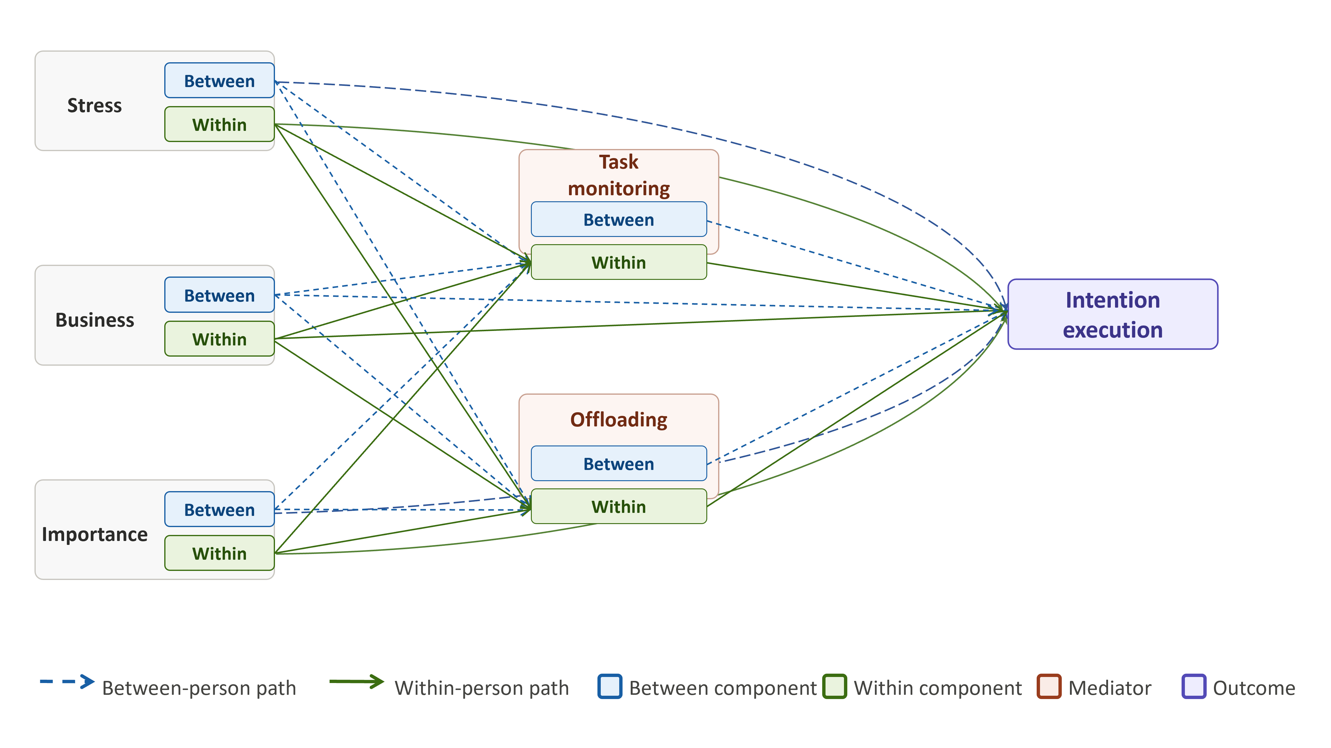
# first, we predict PM from all the predictors
PM_model <-bf(esm_evening_intention_execution ~  # fixed effects 
                within_stress*agegroup.c + 
                within_importance*agegroup.c + 
                within_task_monitoring*agegroup.c + 
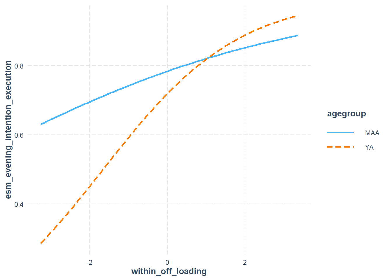
                within_off_loading*agegroup.c +
                within_business*agegroup.c+
                between_stress*agegroup.c + 
                between_task_monitoring*agegroup.c + 
                between_off_loading*agegroup.c +
                between_importance*agegroup.c+
                between_business*agegroup.c+day.c+
                (1 + within_stress +
                   within_business+
                   within_importance + 
                   within_task_monitoring + 
                   within_off_loading || ID), # random intercepts and slopes
              family = bernoulli()) # we have a binary outcome

# predicting monitoring from stress and importance
monitoring_model<- bf(esm_day_task_monitoring ~ 
                        within_stress*agegroup.c +
                        within_importance*agegroup.c +
                        within_business*agegroup.c+
                        between_stress*agegroup.c+
                        between_importance*agegroup.c+
                        between_business+day.c+
                        (1+within_stress+
                           within_business+
                           within_importance+
                           day.c||ID), 
                      family = bernoulli()) # mixture

# predicing off_loading from stress and imortance
offloading_model<-bf(esm_evening_off_loading_r ~ 
                       within_stress*agegroup.c +
                       within_importance*agegroup.c+
                       within_business*agegroup.c+
                       between_stress*agegroup.c+
                       between_importance*agegroup.c+
                       between_business*agegroup.c+ day.c+
                       (1+within_stress+
                          within_importance+
                          within_business+
                          day.c||ID), family = bernoulli() )#

# set weakly informative priors
priors <- c(
  # Fixed effects: assume standardized predictors
  prior(normal(0, 0.5), class = "b", resp = "esmeveningintentionexecution"),   
  prior(normal(0, 0.5), class = "b", resp = "esmdaytaskmonitoring"),  
  prior(normal(0, 0.5), class = "b", resp = "esmeveningoffloadingr")   
  
# all the rest is left as defauls
 #  
 #  # SD of random effects (hierarchical structure)
 #   prior( student_t(3, 0, 2.5) , class = "sd", resp = "esmeveningintentionexecution"),
 #  prior(student_t(3, 0, 2.5) , class = "sd", resp = "esmdaytaskmonitoring"),
 #   prior(student_t(3, 0, 2.5), class = "sd", resp = "esmeveningoffloadingr"),
 #  #
 #  # Correlation priors among random effects
 # # prior(lkj(2), class = "cor"),  # same across responses
 # 
 #  # Residual SDs for continuous outcomes
 #  prior(exponential(1), class = "sigma", resp = "esmdaytaskmonitoring"),
 #  prior(exponential(1), class = "sigma", resp = "esmeveningoffloadingr")
)


# fit the model
fit1 <- brm(
  PM_model+
    monitoring_model + 
    offloading_model + 
    set_rescor(F), 
  prior = priors,
  sample_prior = "yes",
  data = stress_int_red,
  chains = 4, cores = 4,
  iter = 2000, 
  warmup = 1000

)

Posterior summary

Path model results

Moderation of Age group on between stress-within task monitoring path

Code

int_mod_stess_mon<-glmer(esm_day_task_monitoring~between_stress*agegroup +(1|ID),
               family = binomial(),
               data = stress_int_red, )


tab_model(int_mod_stess_mon)

	esm_day_task_monitoring
Predictors	Odds Ratios	CI	p
(Intercept)	0.59	0.49 – 0.71	<0.001
between stress	0.69	0.58 – 0.83	<0.001
agegroup [YA]	1.09	0.83 – 1.42	0.536
between stress × agegroup [YA]	2.08	1.57 – 2.76	<0.001
Random Effects
σ²	3.29
τ₀₀ _ID	0.82
ICC	0.20
N _ID	210
Observations	8171
Marginal R² / Conditional R²	0.032 / 0.225

Code

int_mod_stress_mon<-glmer(esm_day_task_monitoring~day.c+ esm_day_stress*agegroup +(1+day.c+esm_day_stress|ID),
               family = binomial(),
               data = stress_int_red )

boundary (singular) fit: see help('isSingular')

Code

tab_model(int_mod_stress_mon)

	esm_day_task_monitoring
Predictors	Odds Ratios	CI	p
(Intercept)	0.52	0.40 – 0.68	<0.001
day c	0.93	0.92 – 0.94	<0.001
esm day stress	1.06	0.97 – 1.17	0.194
agegroup [YA]	0.48	0.34 – 0.69	<0.001
esm day stress × agegroup [YA]	1.36	1.19 – 1.55	<0.001
Random Effects
σ²	3.29
τ₀₀ _ID	0.96
τ₁₁ _ID.day.c	0.00
τ₁₁ _{ID.esm_day_stress}	0.11
ρ₀₁	1.00
	-0.45
N _ID	210
Observations	8171
Marginal R² / Conditional R²	0.049 / NA

Code

interact_plot(int_mod_stress_mon, pred = esm_day_stress, modx = agegroup)

Code

 ggplot(stress_int_red, 
         aes( x=esm_day_stress, y=esm_day_task_monitoring))+
  # add the "smooth" line, which the regression method ('l,')
  # and trasparent (0.5)
    geom_line(stat="smooth",method = "glm", formula=y~x, alpha=0.5, se=F)+

  # specify that we want different colours for different participants
    aes(colour = factor(ID))+
  # add the summary line with geom_smooth
    geom_smooth(method="lm",formula=y~x, se=T, colour = "black" )+
    theme(strip.text.x = element_text(size = 13))+
    theme_classic()+
    theme(panel.spacing = unit(1, "lines"))+
    facet_wrap(.~agegroup)+
    #ggtitle("Experiment 2")+
    theme(legend.position = "none")

Warning: Removed 635 rows containing non-finite outside the scale range
(`stat_smooth()`).
Removed 635 rows containing non-finite outside the scale range
(`stat_smooth()`).

Plot moderation of Age group on between stress-within task monitoring path

Code

interact_plot(int_mod_stess_mon, pred = between_stress, modx = agegroup)

Test the mediation of monitoring

Code

h_business_monitoring<-hypothesis(fit1,  c("esmeveningintentionexecution_within_task_monitoring*esmdaytaskmonitoring_within_business =0"  ))

plot(h_business_monitoring)

Code

print(h_business_monitoring)

Hypothesis Tests for class b:
                Hypothesis Estimate Est.Error CI.Lower CI.Upper Evid.Ratio
1 (esmeveningintent... = 0     0.02      0.01     0.01     0.03       0.18
  Post.Prob Star
1      0.15    *
---
'CI': 90%-CI for one-sided and 95%-CI for two-sided hypotheses.
'*': For one-sided hypotheses, the posterior probability exceeds 95%;
for two-sided hypotheses, the value tested against lies outside the 95%-CI.
Posterior probabilities of point hypotheses assume equal prior probabilities.

Code

print(paste0("Bayes Factor for ", "h_mediation"," is ", 1/h_business_monitoring$hypothesis$Evid.Ratio))

[1] "Bayes Factor for h_mediation is 5.56821630181082"

Test moderated mediation - Age as moderator, off-loading as a mediator

Code

h_moderated_mediation<-hypothesis(fit1,  c("esmeveningintentionexecution_agegroup.c:within_off_loading* esmeveningoffloadingr_within_importance = 0"  ))

BF_moderated_med<-1/h_moderated_mediation$hypothesis$Evid.Ratio
print(paste0("Bayes Factor for ", "h_moderated_mediation"," is ", 1/h_moderated_mediation$hypothesis$Evid.Ratio))

Moderation model

Generalized linear mixed model fit by maximum likelihood (Laplace
  Approximation) [glmerMod]
 Family: binomial  ( logit )
Formula: esm_evening_intention_execution ~ within_off_loading * agegroup +  
    (within_off_loading | ID)
   Data: stress_int_red

      AIC       BIC    logLik -2*log(L)  df.resid 
   9571.4    9620.9   -4778.7    9557.4      8619 

Scaled residuals: 
    Min      1Q  Median      3Q     Max 
-3.6160 -0.9707  0.4621  0.6220  2.0074 

Random effects:
 Groups Name               Variance Std.Dev. Corr  
 ID     (Intercept)        0.43321  0.6582         
        within_off_loading 0.06023  0.2454   -0.42 
Number of obs: 8626, groups:  ID, 210

Fixed effects:
                              Estimate Std. Error z value Pr(>|z|)    
(Intercept)                    1.29017    0.07643  16.880  < 2e-16 ***
within_off_loading             0.23164    0.05461   4.242 2.22e-05 ***
agegroupYA                    -0.34823    0.10549  -3.301 0.000963 ***
within_off_loading:agegroupYA  0.33695    0.08180   4.119 3.80e-05 ***
---
Signif. codes:  0 '***' 0.001 '**' 0.01 '*' 0.05 '.' 0.1 ' ' 1

Correlation of Fixed Effects:
            (Intr) wthn__ aggrYA
wthn_ff_ldn -0.084              
agegroupYA  -0.714  0.081       
wthn_ff_:YA  0.080 -0.606 -0.068

Plot moderation

Code

interact_plot(int_mod, pred = within_off_loading, modx = agegroup)

Code

# # get the posterrior samples
# draws<-posterior_samples(fit1)
# 
# # Compute indirect effect manually
# draws$indirect <- draws$b_withinoffloading_within_importance * # path a - M~A
#   draws$b_esmeveningintentionexecution_within_off_loading  # path b - Y~M

# # plot distribution
# ggplot(draws, aes(x = indirect))+
#   geom_histogram()+
#   theme_classic()+
#   gg_title("posterior distribution indirect effect of intention on PM")

#indirect_bf <- bayesfactor_parameters(draws$indirect)

#plot(bayesfactor_parameters(draws$indirect))

# draws$indirect2 <- draws$b_withintaskmonitoring_within_business*  draws$b_esmeveningintentionexecution_within_task_monitoring 
# 
# 
# hist(draws$indirect)
# 
# hist(draws$indirect2)
# 
# # simple slope analysis for the interaction between age group and within task monitoring
# slope_MA <- draws$b_esmeveningintentionexecution_within_off_loading  +
#   draws$`b_esmeveningintentionexecution_agegroup.c:within_off_loading` * 0.5
# slope_YA <- draws$b_esmeveningintentionexecution_within_off_loading  +
#   draws$`b_esmeveningintentionexecution_agegroup.c:within_off_loading`  -0.5+0.5
# 
# describe_posterior(slope_MA)
# describe_posterior(slope_YA)
# 
# conditional_effects(fit1, "within_off_loading", resp = "esmeveningintentionexecution")
# 
# ce <- conditional_effects(fit1, effects = "within_off_loading:agegroup.c",
#                           conditions = data.frame(agegroup.c = c(-0., 0.52)))
# 
# plot(ce)

# stronger in young adults than in middle aged adults

Posterior predictive check

PPC constructs the posterior distribution over the parameters and simulate their distribution - if it approximates the distribution of observed data, the model is a good fit

Prospective memory

Code

pp_check(fit1, resp = "esmeveningintentionexecution")

Using 10 posterior draws for ppc type 'dens_overlay' by default.

Posterior predictive check

Task Monitoring

Code

pp_check(fit1, resp = "esmdaytaskmonitoring")

Using 10 posterior draws for ppc type 'dens_overlay' by default.

Posterior predictive check

Off Loading

Code

pp_check(fit1, resp = "esmeveningoffloadingr")

Using 10 posterior draws for ppc type 'dens_overlay' by default.